Data bases
Part 2. Indexes and keys
Part 3. Joins
Part 4. Stored Procedures and Triggers
Part 5. Transactions
Part 6. Normalization and optimization
Just as a strong foundation is crucial for any endeavor, understanding basic SQL concepts is vital for efficient data management. SQL, or Structured Query Language, serves as your bridge to organizing, retrieving, and manipulating data. Whether you're a developer or data enthusiast, these core SQL topics lay the groundwork for your journey into databases.
In this section, we'll uncover key SQL concepts. We'll break down the language and illustrate concepts with examples, making it easy for you to build queries, filter data, and get better results. Let's dive in and build a solid foundation for your SQL skills.
Basic SQL query structure
SQL, or Structured Query Language, is a versatile tool encompassing both Data Definition Language (DDL) and Data Manipulation Language (DML) statements. These statements form the core of SQL's functionality, allowing you to manage both the structure and contents of a database.
Data Definition Language (DDL): DDL statements such as CREATE, ALTER, and DROP focus on the schema of a database. The CREATE statement forms new tables, indexes, or other database objects. ALTER modifies existing schema elements, while DROP deletes them. DDL commands provide the foundation for database design and structure.
Data Manipulation Language (DML): On the other hand, DML statements like SELECT, INSERT, UPDATE, and DELETE enable you to interact with the data within tables. The SELECT statement retrieves specific data, while INSERT adds new records. UPDATE modifies existing data, and DELETE removes records. DML operations are at the heart of working with the actual content of your database.
What is SQL function
In the world of SQL, a function is like a mini-program that performs specific tasks on your data. Just as a calculator helps you crunch numbers; SQL functions help you process data in your database.
Why Use Functions?
Functions are handy because they save time and effort. Instead of writing long and complex queries every time, you can use a function to do the work for you.
Common SQL Functions
COUNT(): This function counts the number of rows in a table. Like counting people in a room, it tells you how many records you have.

SUM(): It adds up numbers in a column. Imagine calculating the total money spent by customers.

AVG(): This calculates the average of numbers. Useful for finding average test scores.
SELECT AVG(score) FROM Exams;
MIN() and MAX(): They find the smallest and largest values. Like picking the shortest and tallest person in a group.
SELECT MIN(price), MAX(price) FROM Products;
UPPER() and LOWER(): These change text to uppercase or lowercase. Useful for consistent formatting.
SELECT UPPER(name) FROM Students;
CONCAT(): It combines text from different columns. Think of it as gluing words together.
SELECT CONCAT(first_name, ' ', last_name) FROM Employees;
Analytic SQL Functions:
Analytical functions allow the user to calculate an aggregate value depending on the grouping of rows. These functions differ from the aggregate functions as they return multiple rows for each group. The rows returned are known as windows that the analytic_clause can define.
An analytical function may take 0-3 argument values. The arguments entered in the functions can be numerical values or non-numeric data types that can be changed into numeric data types.
OVER is an analytic_clause the user uses to indicate that the analytical function mentioned is implemented on a query result set. Once the FROM, WHERE, GROUP BY, and HAVING clauses are executed, this clause is implemented. The user can specify the analytic functions with an OVER clause in the list or using the ORDER BY clause. These clauses enable the user to filter the results generated by implementing the analytic function. It allows one to nest these functions in a parent query and then filter the results of the nested subqueries in the SQL.
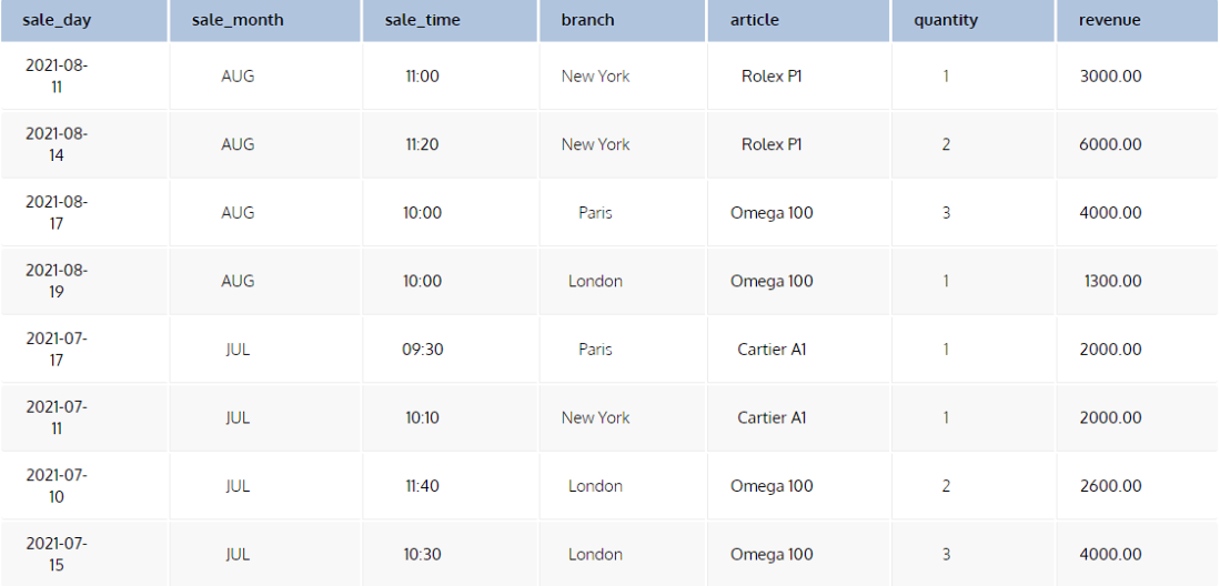
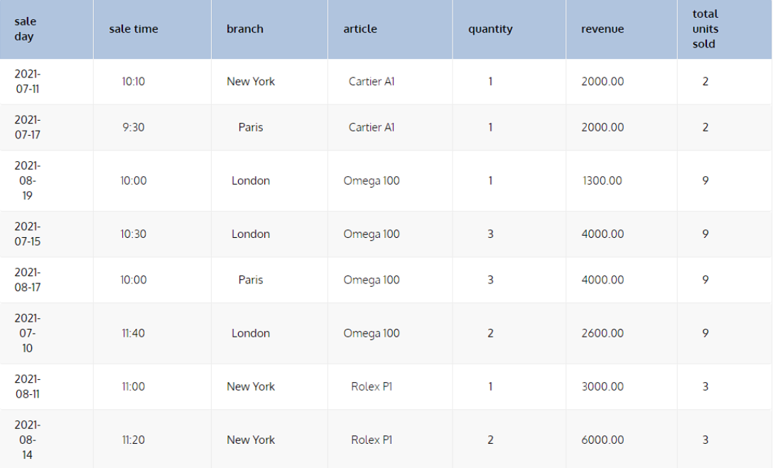
For example, we have a Sales table:
Let’s see the SQL OVER clause in action. Here’s a simple query that returns the total quantity of units sold for each article.
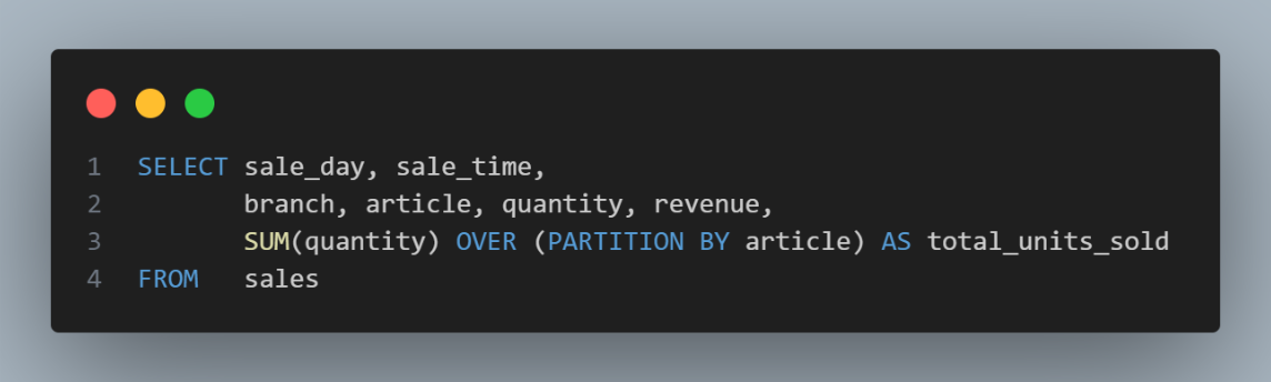
This query will show all the records of the sales table with a new column displaying the total number of units sold for the relevant article. We can obtain the quantity of units sold using the SUM aggregation function, but then we couldn’t show the individual records.
In this query, the OVER PARTITION BY article subclause indicates that the window frame is determined by the values in the article column; all records with the same article value will be in one group. Below, we have the result of this query:
SQL Cursors
What is SQL Cursor?
In the realm of SQL, a cursor is like a virtual pointer that allows you to traverse through the rows of a result set one by one. Just as you might read a book page by page, SQL cursors let you process data step by step.
Why Use Cursors?
Cursors are useful when you need to interact with data in a row-by-row manner. They come in handy for tasks like complex data manipulation or performing actions on specific records.
Using SQL Cursors:
DECLARE Cursor:
First, you declare a cursor and associate it with a SELECT statement. This sets the stage for your data traversal.
DECLARE example_cursor CURSOR FOR
SELECT name, age FROM Employees;
OPEN Cursor:
Next, you open the cursor, making it ready to fetch data. It's like opening a book to start reading.
OPEN example_cursor;
FETCH Data:
Now, you fetch data row by row using the cursor. Think of it as turning pages to read each line.
FETCH NEXT FROM example_cursor INTO @employee_name, @employee_age;
CLOSE Cursor:
Once you've processed all the rows, you close the cursor. It's like closing the book after you've finished reading.
CLOSE example_cursor;
DEALLOCATE Cursor:
Finally, you deallocate the cursor to release resources. It's akin to returning the book to the library.
DEALLOCATE example_cursor;
Example
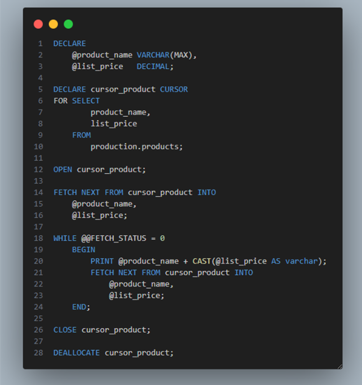
Let`s consider we have a table of Products
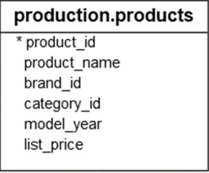
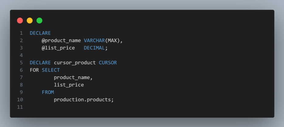
First, declare two variables to hold product name and list price, and a cursor to hold the result of a query that retrieves product name and list price from the PRODUCTS table:
Next, open the cursor:

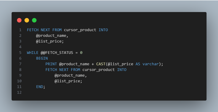
Then, fetch each row from the cursor and print out the product name and list price:
After that, close the cursor:

Finally, deallocate the cursor to release it.

The result:
varchar(n) vs nvarchar(n) vs nvarchar(max)
When it comes to storing text data in a SQL database, understanding the differences between VARCHAR(N), NVARCHAR(N), and NVARCHAR(MAX) is essential. These data types dictate how your text is stored, taking into account character encoding, storage size, and performance considerations.
VARCHAR(N):
- VARCHAR stands for "variable-length character."
- It stores non-Unicode character data with a specified maximum length (N).
- The storage size is Data length + 2 bytes
- Suitable for storing non-Unicode text, like English or numbers.
NVARCHAR(N):
- NVARCHAR stands for "national variable-length character.
- It stores Unicode character data, which supports various languages and character sets.
- The storage size is 2 * Data length + 2 bytes
- Useful for multilingual or international applications that require Unicode support.
NVARCHAR(MAX):
- Similar to NVARCHAR(N) but optimized for storing large amounts of text data.
- Storage size varies based on the length of the data, with a maximum of 2 GB.
- Ideal for storing lengthy text, such as articles, comments, or descriptions.
- Cannot create indexes directly on NVARCHAR(MAX) columns. However, alternative indexing methods like filtered indexes or full-text indexing can be used to enhance search performance.
Choosing the Right Data Type:
- Use VARCHAR(N) for non-Unicode text with a specific length limit, optimizing storage.
- Use NVARCHAR(N) for Unicode support and when you know the data won't exceed a certain length.
- Use NVARCHAR(MAX) for accommodating substantial amounts of text data.
What if we specify n in nvarchar(n) greater than maximum?
If you specify a value of N in NVARCHAR(N) that exceeds the maximum storage capacity, the excess data will be stored separately as "text", while the main table will hold a reference to it. This optimizes storage and maintains query performance.
Let's say you have an NVARCHAR(150) column meant for storing comments. If you specify N as 150 and someone enters a comment of 200 characters, the extra 50 characters will not be directly stored in the column. Instead, they will be stored as "text" outside the main table, and the column in the main table will have a reference to this external storage.
This benefits both storage and performance. Your main table doesn't need to reserve unnecessary space for infrequent long comments, and querying remains efficient because the main table only retrieves the referenced "text" data when needed.
View/Materialized View
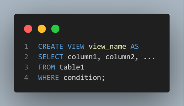
View: A view in a database is a virtual table created by executing a SELECT query against one or more existing tables. It presents the data from those tables in a structured and customized manner without actually storing the data itself. Views allow you to abstract complex queries and present a simplified, tailored view of the data to users or applications.
Example:
Let's say you have two tables: Customers and Orders. You want to create a view that displays customer names along with their order counts.
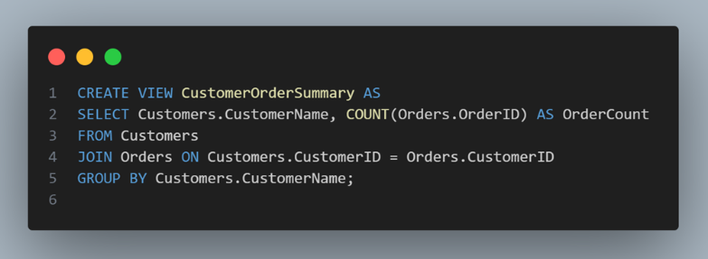
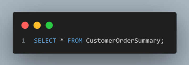
After executing this SQL statement, you'll have a view named CustomerOrderSummary that you can query just like a regular table:
Materialized View: A materialized view (or materialized query table) takes the concept of a view a step further by physically storing the result set of a query. This storage enables faster access to the data as it eliminates the need to recompute the result each time the view is accessed. Materialized views are particularly beneficial for complex or resource-intensive queries.
Differences:
- Storage: Views don't store data; materialized views store precomputed data. Views are not physically stored on the disk and so, each time it gets updated when accessed while on the other hand, Materialized Views are directly stored on the disc.
- Performance: Materialized views offer faster query performance due to precomputed data.
- Query Complexity: Materialized views optimize complex queries involving aggregations or joins.
- Data Freshness: Views always reflect real-time data; materialized views need periodic refreshing.
- Use Cases: Views simplify data access; materialized views optimize query performance and analysis.